
Neural Networks
(Many are copied from Sun, 2019 Optimization paper)
Optimization
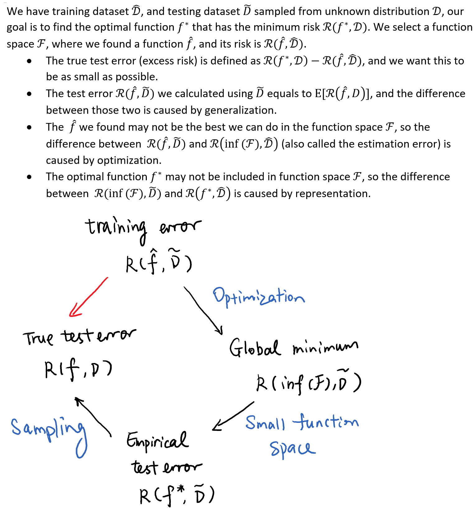 So, even if we find the global minimum of the loss function (no estimzation error) and the optimal classcification boundary is learnable by the network (function space is large enough so that there are no approximation error), the loss function is just a proxy for the classcification error, the minimum for the loss is not the best boundary.(we still have the error caused by sampling).
Gradient descents and its variants:
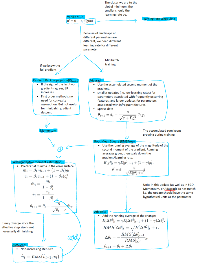
Momentum
- Keeps a running average of the gradient, usually keeps to be 0.9old, 0.1new.
- Move more to the direction with more loss drop. If the direction oscilates, then the running average should be small. Then move less to that direction.
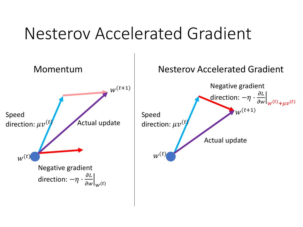
- Nestorov’s accelerated gradient: first extended the previous step and calcualted the gradient at the new place.
Some learning rate scheduling techniques
- Vanilla SGD: divide the step-size by a fixed constant once every few epochs or divide by a constant when stuck.
- Learning rate warmup: Commonly used heuristic in deep learning. Use a very small learning rate for a number of iterations, and then increases to the “regular” .
- Cyclical learning rate: Let the step-size bounce between a lower threshold and an upper threshold. Restart: decreases to the lower threshold and suddenly increases to the upper threshold.
Convergence
- One dimensional: we can diverge if \(\eta \ge 2 \eta_{opt}\)
- Multi-variant: learning rate is the same for all dimension, we can diverge if \(\eta \ge 2 min_i \eta_{i,opt}\)
- Convergence is slow when condition number of the Hessian (ratio of largest to smallest eigenvalue) is small(0402200, I think this might be wrong? It should be the opposite, large condiction number is bad for convergence)
- It can be stuck at saddle points(more common than local optimal)
- The nn is a high bias low variance classcifier.(Outlier would not change the boundary.) But perceptron learning rule is sensitive to outliers.
Newton’s method
- Difficult to invert(too large)
- Not convex function hessian are not psd
- Use quasi-newton’s method.
- Less popular for large nn
- Quickprop: partial second derivative at one direction (Treats each dimension seperately). Quickprop assumes the error surface to be locally quadratic and attempts to jump in one step from the current position directly into the minimum of the parabola.
Initialization
The general idea is making the variance of the output close to 1. We usually normalize the input variance to be zero mean and variance 1 and the mean of the weights are initialized to be 0, and based on this, the variance of the weights can be calcualted.
- LeCun and Xavier initialization: More suitable for linear/sigmoid activation. LeCun only thinks about the influence of the forward pass, so \(Var(w) = 1/fanIn\), and Xavier considers both forward and backward pass, so \(Var(w) = \frac{2}{fanIn+fanOut}\)
- Kaiming initialization: ReLU activation was used, so \(Var(w) = 2/fanIn\) or \(Var(w) = 2/fanOut\)
- Dynamical isometry: This line of research looks at the the singular values of the input-output Jacobian matrix and trying to make that all 1. (My understanding is that in this way, the gradient of output over input is on the same scale, so we can use one learning rate to update all teh output feature and have a good, stable reasult). We could use all orthogonal matrices as the inilization weights for sigmoid activation, but dynamical isometry properity cannot be observed if using orthogonal matrices and ReLU.
- Computing spectrum: This is a way to evaluate the performance of the training. We can look at the Hessian matrix or even the weights parameters. By looking at the Hessian of ImageNet, it verified that the local Lipschitz constant of the gradient (the maximum eigenvalue of the Hessian) is rather small in practical neural network training(? Paper Sun, 2019 says like it is a good thing, is it?), partially due to careful initialization.
Normalization
We want the “preactivation/input” matrix to have zero mean and unit variance for each feature. This is a pre-conditioning technique that can reduce the condition number of the Hessian matrix.
Batch normalization
- Added before non-linear activation function.
- For each feature (i.e. each pixel for a image), calculate its mean ##\mu## and variance ##\sigma##, then calculate \(\eta \times \frac{x-\mu}{\sigma + \epsilon} + \beta\), where \(\eta\) and \(\beta\) are learnable parameters
- It can reduce the “internal covariate shift”, reduce the Lipschitz constants (of the objective and the gradients), allow larger learning rate, remove large isolated eigenvalues.
- If different mini-batches do not have similar statistics then BN does not work very well.
Other input normalization methods
For a input matrix of size num_feature \(\times\) batch_size, BatchNorm chooses to normalize cross rows (more precisely, divide each row into many segments and normalize each segment), layer normalization normalizes the columns, and group normalization normalizes a sub-matrix that consists of a few columns and a few rows
Weights normalization methods
Weight normalization separates the norm and the direction of the weight matrix. Spectral normalization divided the weight matrix by its spectral norm of W.