Approximate Inference

(Summarized from the lecture notes from cmu spring17-10708, Eric Xing)

Motivation

When we want to know $E_p[f(x)]$, where $x \sim p(x)$, we need to know the distribution of $x$. One way is to use a sampled base average to approximate the expectation $E_p[f(x)] = \frac{1}{N} \sum_{t=1}^{N}f(x^{(t)})$. However a few challenges remain that:

• how to draw samples from a given dist. (not all distributions can be trivially sampled)?
• how to make better use of the samples (not all sample are useful, or eqally useful, see an example later)?
• how to know we’ve sampled enough? (For a model with hundreds or more variables, rare events will be very hard to garner evough samples even after a long time or sampling)

So we have a few methods belong to the Monte Carlo methods:

• Rejection sampling: Create samples like direct sampling, only count samples which is consistent with given evidences.
• Likelihood weighting: Sample variables and calculate evidence weight. Only create the samples which support the evidences.
• Markov chain Monte Carlo (MCMC): Metropolis-Hasting, Gibbs

Rejection sampling:

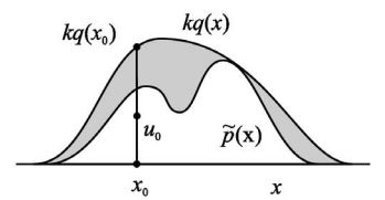
How to generate samples given a distribution $p(x)$? How to convert samples from a Uniform[0,1] generator to samples that follows distribution $p(x)$? One way is to compute cdf $h(y)$, which is a uniform non-decreasing function in [0,1]. Then for every sample $u$ from Uniform[0,1], we can get $x = h^{-1}(u)$ that $x \sim p(x)$. But this won’t work if $\hat{p}(x)$ is not normalized (assume $p(x) = \frac{\hat{p}(x)}{Z}$). This leads to the idea of rejection sampling:

1. Come up with a probability distribution $Q(x)$ (usually Gaussian) that we can easily draw samples from.
2. Find a constant $k$ such that $\frac{\hat{p}(x)}{kQ(x)} < 1$.
3. Draw a sample $x_0$ from $Q$
4. Accept a sample with probability $\frac{\hat{p}(x)}{kQ(x)}$: sample $u_0$ from Uniform[0,$kQ(x_0)$], accept the sample if $u_0 < \hat{p}(x_0)$

And it can be proved that the accpected samples follows $p(x)$.

Pitfalls:

• Scale badly with dimensionality (acceptance rate exponentially decreases)
• If $Q(x)$ is chosen badly (if $p$ and $Q$ both are Gaussian), acceptance rate is really low

Importance sampling:

A different idea is to retain all the samples and re-weight them while computing their mean. $E_p[f(x)] = \int f(x)p(x)dx = \int f(x) \frac{p(x)}{q(x)}q(x)dx \approx \frac{1}{N} \sum_{n=1}^{N} f(x^{(n)}) \frac{p(x^{(n)})}{q(x^{(n)})}$, where $x^{(n)} \sim q(x)$. This a an unbiased estimator. However, when we only have unnormalized distribution $\hat{p}(x)$, $E_p[f(x)] \approx \sum_{n} f(x^{(n)})w^{(n)}$, where $w^{(n)} = \frac{\hat{p}(x^{(n)})}{\hat{q}(x^{(n)})}\Big/\sum_l \frac{\hat{p}(x^{(l)})}{\hat{q}(x^{(l)})}$. This is biased.

Pitfalls:

• Scale badly with dimensionality
• Unless $p$ is close $q$ ($p=q$ gives the best performance), there will be a small number of dominant weights leading to a high variance. This is particularly evident in high-dimensions
• This problem can be alleviated by resampling the weights

Weighted resampling

1. Draw $N$ samples $\{x\}_N$ from $Q$
2. Constructing weights: $w^{(n)} = \frac{\hat{p}(x^{(n)})}{\hat{q}(x^{(n)})}\Big/\sum_l \frac{\hat{p}(x^{(l)})}{\hat{q}(x^{(l)})}$
3. Subsample $x$ from $\{x\}_N$ w.p.t. $\{w\}_N$

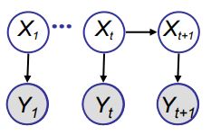
Particle filters

• Apply the resampled importance sampling to a temporal high dimensional distribution $p(x_1, \dots, x_t)$. The problem can be reduced to finding a proposal distribution for an one-dimensional problem.
• Goal is to yield samples from posterior $p(X_t|Y_{1:t})$

Markov Chain Monte Carlo

Instead of using a fixed proposal $Q(x)$ as the previous methods, we use $Q(x^{\prime} | x)$ where $x^{\prime}$ is the new state being sampled, and $x$ is the previous sample. So as $x$ changes, $Q(x^{\prime} | x)$ can also change. One of the most famous MCMC algorithm is Metropolis-Hastings algorithm.

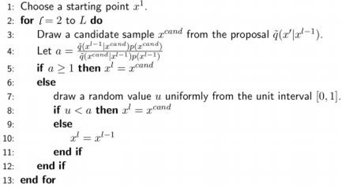
Metropolis-Hastings

• Draws a sample $x^{\prime}$ from $Q(x^{\prime} ; x)$
• The new sample $x^{\prime}$ is accepted or rejected with some probability $A(x^{\prime} ; x)$
  • This acceptance probability is $A(x^{\prime} ; x) = \min(1, \frac{p(x^{\prime})Q(x ; x^{\prime})}{p(x)Q(x^{\prime} ; x)})$
  • $A(x^{\prime} ; x)$ is like a ratio of importance sampling weights
    • $p(x^{\prime})Q(x ; x^{\prime})$ is the importance weight for $x^{\prime}$, $p(x)Q(x^{\prime} ; x)$ is the importance weight for x.
    • We divide the importance weight for $x^{\prime}$ by that of $x$
    • Notice that we only need to compute $p(x^{\prime})/p(x)$ rather than $p(x^{\prime})$ or $p(x)$ separately
  • $A(x^{\prime} ; x)$ ensures that, after sufficiently many draws, our samples will come from the true distribution.

Steps for the algorithm:

First we have a burn-in stage: while samples have not converged, do: Then, we take samples using the same procedure as above, and keep those samples.

Gibbs sampling

Gibbs Sampling is an MCMC algorithm that samples each random variable of a graphical model, one at a time. GS is a special case of the MH algorithm.